(二)OpenCV |
您所在的位置:网站首页 › 增强亮度 含义成语 › (二)OpenCV |
(二)OpenCV
|
·对于部分图像,会出现整体较暗或较亮的情况,这是由于图片的灰度值范围较小,即对比度低。实际应用中,通过绘制图片的灰度直方图,可以很明显的判断图片的灰度值分布,区分其对比度高低。对于对比度较低的图片,可以通过一定的算法来增强其对比度。常用的方法有线性变换,伽马变换,直方图均衡化,局部自适应直方图均衡化等。
1. 灰度直方图及绘制
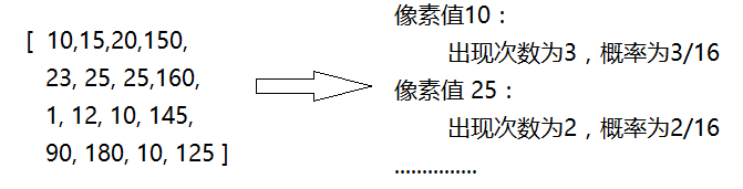
灰度直方图用来描述每个像素在图像矩阵中出现的次数或概率。其横坐标一般为0-255个像素值,纵坐标为该像素值对应的像素点个数。如下图所示的图像矩阵(单通道灰度图,三通道时可以分别绘制),可以统计每个像素值出现的次数,也可以统计概率,统计像素值出现次数的灰度直方图如下所示。 灰度直方图绘制 a, 可以利用opencv的calcHist()统计像素值出现次数,通过matploblib的plot()绘制 b, 可以直接利用matploblib的hist()方法 cv2.calcHist() 参数: img:输入图像,为列表,如[img] channels: 计算的通道,为列表,如[0]表示单通道,[0,1]统计两个通道 mask: 掩模,和输入图像大小一样的矩阵,为1的地方会进行统计(与图像逻辑与后再统计);无掩模时为None histSize: 每一个channel对应的bins(像素值)个数,为列表,如[256]表示256个像素值 ranges: bins的边界,为列表,如[0,256]表示像素值范围在0-256之间 accumulate: Accumulation flag. If it is set, the histogram is not cleared in the beginning when it is allocated. This feature enables you to compute a single histogram from several sets of arrays, or to update the histogram in time.如下图所示,分别绘制了灰度分布曲线图,灰度分布直方图和两者叠加图形,代码如下: View Code #coding:utf-8 import cv2 as cv import matplotlib.pyplot as plt import numpy as np img = cv.imread(r"C:\Users\Administrator\Desktop\maze.png",0) hist = cv.calcHist([img],[0],None,[256],[0,256]) plt.subplot(1,3,1),plt.plot(hist,color="r"),plt.axis([0,256,0,np.max(hist)]) #piot.plot表示线条颜色红色; plt.axis([a,b,c,d]) 设置x轴的范围为【a,b】 y轴的范围为【c,d】 plt.xlabel("gray level") #x轴的名字标签 plt.ylabel("number of pixels") #y轴的标签 plt.subplot(1,3,2),plt.hist(img.ravel(),bins=256,range=[0,256]),plt.xlim([0,256]) #plt.hist(src,pixels) src:数据源,注意这里只能传入一维数组,使用src.ravel()可以将二维图像拉平为一维数组。pixels:像素级,一般输入256。 plt.xlabel("gray level") plt.ylabel("number of pixels") plt.subplot(1,3,3) plt.plot(hist,color="r"),plt.axis([0,256,0,np.max(hist)]) plt.hist(img.ravel(),bins=256,range=[0,256]),plt.xlim([0,256]) plt.xlabel("gray level") plt.ylabel("number of pixels") plt.show()
c.通过np.histogram()和plt.hist()也可以计算出灰度值分布 #coding:utf-8 import cv2 as cv import matplotlib.pyplot as plt import numpy as np img = cv.imread(r"C:\Users\Administrator\Desktop\maze.png",0) histogram,bins = np.histogram(img,bins=256,range=[0,256])#a是待统计数据的数组;bins指定统计的区间个数;range是一个长度为2的元组,表示统计范围的最小值和最大值,默认值None,表示范围由数据的范围决定,weights为数组的每个元素指定了权值,histogram()会对区间中数组所对应的权值进行求和,density为True时,返回每个区间的概率密度;为False,返回每个区间中元素的个数 print(histogram) plt.plot(histogram,color="g") plt.axis([0,256,0,np.max(histogram)]) plt.xlabel("gray level") plt.ylabel("number of pixels") plt.show() np.histogram() import cv2 as cv import matplotlib.pyplot as plt import numpy as np img = cv.imread(r"C:\Users\Administrator\Desktop\maze.png",0) rows,cols = img.shape hist = img.reshape(rows*cols) histogram,bins,patch = plt.hist(hist,256,facecolor="green",histtype="bar") #histogram即为统计出的灰度值分布 plt.xlabel("gray level") plt.ylabel("number of pixels") plt.axis([0,255,0,np.max(histogram)]) plt.show() 2. 对比度增强对比度增强,即将图片的灰度范围拉宽,如图片灰度分布范围在[50,150]之间,将其范围拉升到[0,256]之间。这里介绍下 线性变换,直方图正规化,伽马变换,全局直方图均衡化,限制对比度自适应直方图均衡化等算法。 2.1 线性变换 通过函数y=ax+b对灰度值进行处理,例如对于过暗的图片,其灰度分布在[0,100], 选择a=2,b=10能将灰度范围拉伸到[10, 210]。可以通过np或者opencv的convertScaleAbs()函数来实现,对应参数列表如下: cv2.convertScaleAbs(src,alpha,beta) src: 图像对象矩阵 dst:输出图像矩阵 alpha:y=ax+b中的a值 beta:y=ax+b中的b值 (对于计算后大于255的像素值会截断为255)使用示例代码和效果图如下: convertScaleAbs() #coding:utf-8 import cv2 as cv import matplotlib.pyplot as plt import numpy as np img = cv.imread(r"C:\Users\Administrator\Desktop\dark.jpg") print(img) img_bright = cv.convertScaleAbs(img,alpha=1.5,beta=0) print(img_bright) cv.imshow("img",img) cv.imshow("img_bright",img_bright) cv.waitKey(0) cv.destroyAllWindows()numpy实现 #coding:utf-8 import cv2 as cv import matplotlib.pyplot as plt import numpy as np img = cv.imread(r"C:\Users\Administrator\Desktop\dark.jpg") a=1.5 b=0 y = np.float(a)*img+b y[y>255]=255 y = np.round(y) #round( x [, n] ) 返回 x 的小数点四舍五入到n个数字。 img_bright= y.astype(np.uint8) #输出图像在类型是8字节 cv.imshow("img",img) cv.imshow("img_bright",img_bright) cv.waitKey(0) cv.destroyAllWindows()(实用性:numpy自定义实现时,可以针对不同区间像素点,采用不同系数a,b来动态改变像素值)
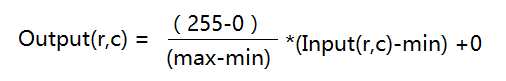
2.2 直方图正规化 对于上述线性变换,系数a,b需要自己摸索设置。但是直方图正规化的系数固定,一般将原图片的像素值范围映射到[0,255]范围内。假设原图片的像素值分布范围为Input:[min, max], 映射后的范围为Output:[0,255], 则对应的系数a=(255-0)/(max-min), 系数b=0。即计算公式:
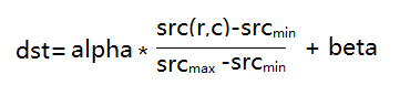
opencv提供了normalize()函数来实现灰度正规化,对应参数列表如下: cv2.normalize(src,dst,alpha,beta,normType,dtype,mask) 参数: src: 图像对象矩阵 dst:输出图像矩阵(和src的shape一样) alpha:正规化的值,如果是范围值,为范围的下限 (alpha – norm value to normalize to or the lower range boundary in case of the range normalization.) beta:如果是范围值,为范围的上限;正规化中不用到 ( upper range boundary in case of the range normalization; it is not used for the norm normalization.) norm_type:normalize的类型 cv2.NORM_L1:将像素矩阵的1-范数做为最大值(矩阵中值的绝对值的和) cv2.NORM_L2:将像素矩阵的2-范数做为最大值(矩阵中值的平方和的开方) cv2.NORM_MINMAX:将像素矩阵的∞-范数做为最大值 (矩阵中值的绝对值的最大值) dtype: 输出图像矩阵的数据类型,默认为-1,即和src一样 mask:掩模矩阵,只对感兴趣的地方归一化(对于alpha的值,不是很清楚含义,经过试验,应该是一个锚点,用像素矩阵中的范数计算出来的比例和alpha相乘,当dtype为cv2.NORM_MINMAX时,其计算公式类似如下:
使用示例代码和效果图如下: cv.normalize() #引用这个函数直接正规化 #coding:utf-8 import cv2 as cv import matplotlib.pyplot as plt import numpy as np img = cv.imread(r"C:\Users\Administrator\Desktop\dark.jpg") img_norm=cv.normalize(img,dst=None,alpha=350,beta=10,norm_type=cv.NORM_MINMAX) cv.imshow("img",img) cv.imshow("img_norm",img_norm) cv.waitKey(0) cv.destroyAllWindows()numpy实现类似normalize #利用正规化原理,跑公式 ```python #coding:utf-8 import cv2 as cv import matplotlib.pyplot as plt import numpy as np img = cv.imread(r"C:\Users\Administrator\Desktop\dark.jpg") out_min=0 out_max=255 in_min = np.min(img) #原图最小像素值 in_max = np.max(img) #原图最大像素值 a=float(out_max-out_min)/(in_max-in_min) b=out_min-a*in_min img_norm = img*a+b #正规化原理公式 img_norm = img_norm.astype(np.uint8) cv.imshow("img",img) cv.imshow("img_norm",img_norm) cv.waitKey(0)
|


【本文地址】
今日新闻 |
推荐新闻 |